Plot a recovery landscape from RRI perturbation-recovery metrics

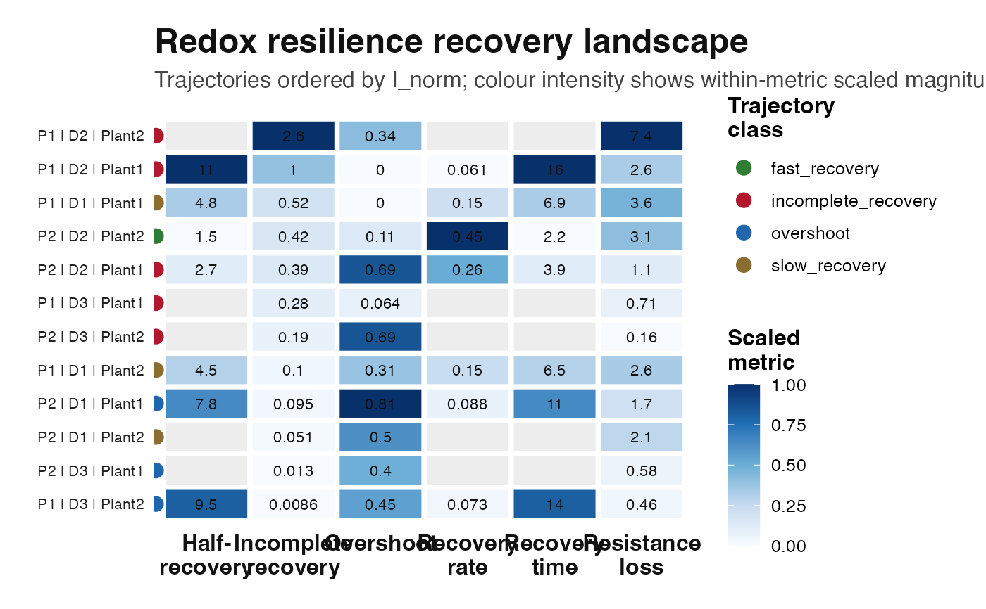
Visualises user-level perturbation-recovery metrics from rri_recovery_metrics(). Each row is one trajectory and each column is a core resilience metric. Values are scaled within metric columns to make amplitudes, overshoot, incomplete recovery, and recovery times comparable.

Usage

plot_rri_recovery_landscape(
  rec,
  group_cols = c("plot", "depth", "plant_id"),
  metrics = c("A_norm", "O_norm", "I_norm", "k", "tau_r", "t_half"),
  order_by = "I_norm",
  base_size = 12
)

Arguments

rec: A data frame returned by rri_recovery_metrics().
group_cols: Character vector identifying trajectory labels.
metrics: Character vector of recovery metric columns to plot.
order_by: Character scalar. Metric used to order trajectories.
base_size: Numeric. Base font size.

Value

A ggplot object.

Examples

sim <- simulate_redox_holobiont(
  n_plot = 2,
  n_depth = 3,
  n_plant = 2,
  n_time = 12,
  p_micro = 20,
  seed = 109
)

res <- rri_pipeline_st(
  ROS_flux = sim$ROS_flux,
  Eh_stability = sim$Eh_stability,
  micro_data = sim$micro_data,
  id = sim$id,
  reducer = "per_domain",
  scaling = "pnorm"
)

rec <- rri_recovery_metrics(
  res = res,
  id = sim$id,
  time_col = "time",
  group_cols = c("plot", "depth", "plant_id"),
  perturb_start = 5,
  perturb_end = 7
)

head(rec)
#>   plot depth plant_id        x0 xmin_perturb xmax_perturb x_extreme
#> 1   P1    D1   Plant1 0.1666895    0.1911321    0.7631028 0.7631028
#> 2   P2    D1   Plant1 0.1441712    0.1501787    0.3859172 0.3859172
#> 3   P1    D2   Plant1 0.2631689    0.0821912    0.9397771 0.9397771
#> 4   P2    D2   Plant1 0.4622820    0.7522711    0.9558848 0.9558848
#> 5   P1    D3   Plant1 0.5581961    0.8904897    0.9563755 0.9563755
#> 6   P2    D3   Plant1 0.6182729    0.8203454    0.9775123 0.9775123
#>   perturb_direction xmin_recovery xmax_recovery       xeq         A    A_norm
#> 1          increase    0.17890974     0.3442096 0.2532884 0.5964133 3.5779889
#> 2          increase    0.02753112     0.2285998 0.1579083 0.2417460 1.6767975
#> 3          increase    0.36015518     0.8505589 0.5381607 0.6766081 2.5710030
#> 4          increase    0.14365060     0.8583562 0.2839480 0.4936028 1.0677524
#> 5          increase    0.52236666     0.8870628 0.7136611 0.3981794 0.7133325
#> 6          increase    0.37181540     0.8182219 0.6261845 0.3592394 0.5810370
#>   tau_lag          O     O_norm           I     I_norm          k         k_r2
#> 1       0 0.00000000 0.00000000 0.086598865 0.51952194 0.14523048 0.0585174941
#> 2       1 0.11664011 0.80903873 0.013737027 0.09528272 0.08836949 0.0478912959
#> 3       0 0.00000000 0.00000000 0.274991791 1.04492492 0.06116515 0.0204734550
#> 4       0 0.31863142 0.68925765 0.178334058 0.38576897 0.25857627 0.1074052966
#> 5       0 0.03582942 0.06418787 0.155465043 0.27851332         NA 0.0005677983
#> 6       0 0.24645750 0.39862252 0.007911643 0.01279636         NA 0.0307292419
#>   k_n                    k_flag     tau_r    t_half  H    trajectory_class
#> 1   5           low_fit_quality  6.885607  4.772739 NA       slow_recovery
#> 2   5           low_fit_quality 11.316123  7.843739 NA           overshoot
#> 3   5           low_fit_quality 16.349178 11.332387 NA incomplete_recovery
#> 4   5           low_fit_quality  3.867331  2.680630 NA incomplete_recovery
#> 5   5 nonpositive_recovery_rate        NA        NA NA incomplete_recovery
#> 6   5 nonpositive_recovery_rate        NA        NA NA           overshoot
plot_rri_recovery_landscape(rec)