Aligned time series with separate physical units — plot_rri

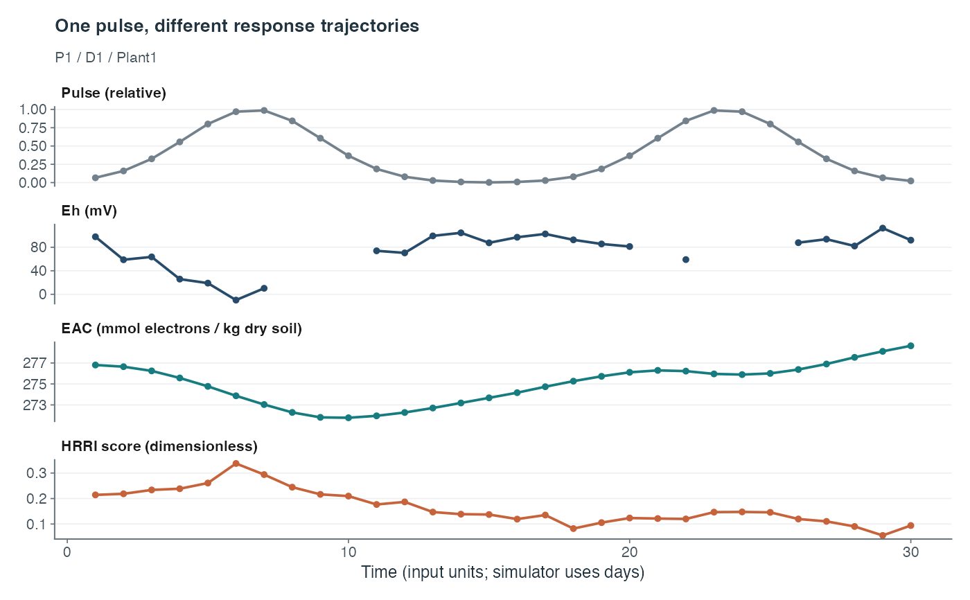
Shows Eh, EAC and the observation-derived score in separate panels sharing time. It does not place unlike units on a common axis.

Usage

plot_rri_timeseries(
  sim,
  res,
  plot_id = "P1",
  depth_id = "D1",
  plant_id = "Plant1",
  perturb_start = NULL,
  perturb_end = NULL,
  base_size = 9,
  forcing = NULL,
  forcing_label = "Pulse (relative)",
  forcing_threshold = NULL,
  time_label = "Time (input units; simulator uses days)"
)

Arguments

sim: Simulator output containing id and soil_data.
res: Pipeline output containing row_scores.
plot_id, depth_id, plant_id: Identifiers for a single trajectory.
perturb_start, perturb_end: Optional disturbance interval in input time units.
base_size: Base font size.
forcing: Optional numeric forcing vector aligned to sim$id; missing values remain gaps. NULL uses simulator event_intensity if available.
forcing_label: Axis label including forcing units.
forcing_threshold: Optional finite scalar marking a declared threshold; it is not inferred from the plotted response.
time_label: Label including input time units.

Value

A ggplot with separate vertically aligned panels, including forcing when supplied or available. Export at approximately 7.4 by 6 inches.

Examples

# \donttest{
  sim <- simulate_redox_holobiont(seed = 1)
  res <- rri_pipeline(soil = sim$Eh_stability, plant = sim$ROS_flux,
                      id = sim$id)
#> Warning: Unanchored latent axes have arbitrary signs; RRI is exploratory, not directionally validated resilience.
#> Warning: Excluding simulator-derived hidden columns from scoring: Cacc_EAC, Cacc_EDC, Cacc_total, Cacc_fraction, net_oxidative_balance, alpha_accept, alpha_donate, k_accept_h, k_donate_h
  plot_rri_timeseries(sim, res)

# }